Energy Injection Scenarios (PDE Solver)

PDE runs for three physically motivated injection histories:

1. Decaying particles — exponential decay of a long-lived relic

2. DM annihilation (s-wave) — \(\langle\sigma v\rangle\) constant

3. DM annihilation (p-wave) — \(\langle\sigma v\rangle \propto v^2 \propto (1+z)\)

The PDE handles continuous injection self-consistently; the distortion at each \(z\) feeds back into DC/BR and \(T_e\).

import numpy as np
import matplotlib.pyplot as plt
from spectroxide import (
    solve, mu_shape, y_shape, delta_n_to_delta_I, cosmic_time, apply_style,
)

apply_style()

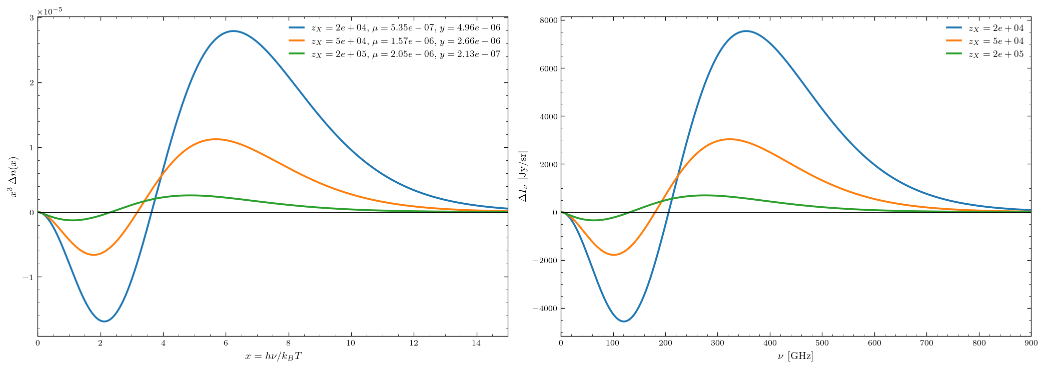
1. Decaying particles

The decay rate \(\Gamma_X\) [s\(^{-1}\)] is the input. To probe a target injection epoch \(z_X\), set \(\Gamma_X = 1/t(z_X)\) so that most decays happen near \(z_X\). Different \(z_X\) probe different regimes: \(z_X > 10^5\) → \(\mu\)-type, \(z_X \sim 5\times 10^4\) → mixed, \(z_X < 10^4\) → \(y\)-type.

z_x_values = [2e4, 5e4, 2e5]
f_x = 5e5  # eV per baryon released

fig, (ax1, ax2) = plt.subplots(1, 2, figsize=(14, 5))

for z_x in z_x_values:
    gamma_x = 1.0 / cosmic_time(z_x)  # Γ_X = 1/t(z_X)
    result = solve(
        injection={'type': 'decaying_particle', 'f_x': f_x, 'gamma_x': gamma_x},
        z_start=5e6, z_end=1e3,
    )
    nu_ghz, dI = delta_n_to_delta_I(result.x, result.delta_n)
    label = f'$z_X = {z_x:.0e}$, $\\mu={result.mu:.2e}$, $y={result.y:.2e}$'
    ax1.plot(result.x, result.x**3 * result.delta_n, lw=1.8, label=label)
    ax2.plot(nu_ghz, dI, lw=1.8, label=f'$z_X = {z_x:.0e}$')

for ax in (ax1, ax2):
    ax.axhline(0, color='k', lw=0.5)
    ax.legend(fontsize=9)
ax1.set(xlabel=r'$x = h\nu / k_B T$', ylabel=r'$x^3 \, \Delta n(x)$', xlim=(0, 15))
ax2.set(xlabel=r'$\nu$ [GHz]', ylabel=r'$\Delta I_\nu$ [Jy/sr]', xlim=(0, 900))
plt.tight_layout()
plt.show()

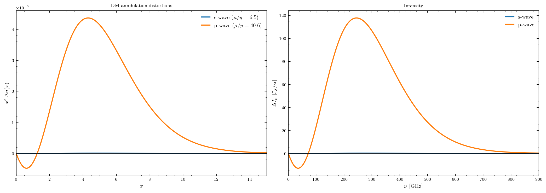
2. DM annihilation: s-wave vs p-wave

	s-wave	p-wave
\(\langle\sigma v\rangle\)	const	\(\propto v^2 \propto (1+z)\)
Heating rate	\(\propto (1+z)^3\)	\(\propto (1+z)^4\)
Distortion	mixed \(\mu + y\)	\(\mu\)-dominated

res_s = solve(injection={'type': 'annihilating_dm', 'f_ann': 2e-23},
               z_start=5e6, z_end=1e3)
res_p = solve(injection={'type': 'annihilating_dm_pwave', 'f_ann': 2e-27},
               z_start=5e6, z_end=1e3)

for name, r in [('s-wave', res_s), ('p-wave', res_p)]:
    print(f'{name}: mu = {r.mu:.3e}, y = {r.y:.3e}, mu/y = {r.mu/r.y:.1f}')

s-wave: mu = 4.693e-10, y = 7.176e-11, mu/y = 6.5
p-wave: mu = 1.544e-07, y = 3.800e-09, mu/y = 40.6

fig, (ax1, ax2) = plt.subplots(1, 2, figsize=(14, 5))

for r, lab in [(res_s, 's-wave'), (res_p, 'p-wave')]:
    ax1.plot(r.x, r.x**3 * r.delta_n, lw=2,
             label=f'{lab} ($\\mu/y = {r.mu/r.y:.1f}$)')
    nu, dI = delta_n_to_delta_I(r.x, r.delta_n)
    ax2.plot(nu, dI, lw=2, label=lab)

for ax in (ax1, ax2):
    ax.axhline(0, color='k', lw=0.5)
    ax.legend(fontsize=10)
ax1.set(xlabel=r'$x$', ylabel=r'$x^3 \, \Delta n(x)$', xlim=(0, 15),
        title='DM annihilation distortions')
ax2.set(xlabel=r'$\nu$ [GHz]', ylabel=r'$\Delta I_\nu$ [Jy/sr]', xlim=(0, 900),
        title='Intensity')
plt.tight_layout()
plt.show()

Summary

Scenario	injection dict
Decaying particle	{'type': 'decaying_particle', 'f_x': ..., 'gamma_x': ...}
s-wave DM	{'type': 'annihilating_dm', 'f_ann': ...}
p-wave DM	{'type': 'annihilating_dm_pwave', 'f_ann': ...}

s-wave gives mixed \(\mu+y\); p-wave is nearly pure \(\mu\). Decay lifetime sets injection epoch.

Next: 03_new_physics.ipynb — dark photon oscillation, monochromatic photon injection.